Do I paste a whole LaTeX document?
No. Paste the tikzpicture environment only; the renderer supplies the document around it. A \usetikzlibrary line at the top of what you paste is loaded too, so positioning, arrows.meta and the other libraries work.
Tools · TikZ
Paste a tikzpicture, press Draw, and get it typeset by LaTeX with TikZ, the same engine Forma draws its own figures with. Download the result as SVG for the web or PNG for slides.
Or describe it in words and get source you can edit, checked before you see it.
Part of Forma Visuals: Draw a technical or research figure · Draw a geometry figure
Flowchart A login flowchart with start and end terminals, an input step and two decisions, built from TikZ node styles (shapes.geometric), relative positioning and arrows.meta tips.
In your browser, drawn with Plotly.js (MIT), Apache ECharts (Apache-2.0, notice), Chart.js (MIT).
01 Examples
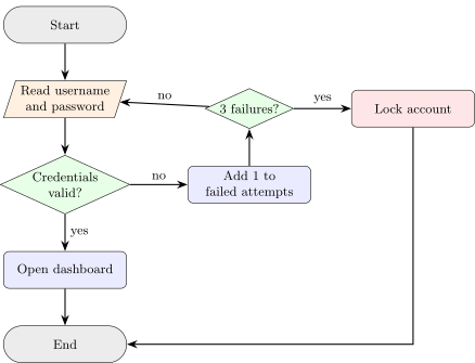
A login flowchart with start and end terminals, an input step and two decisions, built from TikZ node styles (shapes.geometric), relative positioning and arrows.meta tips.
\usetikzlibrary{shapes.geometric, arrows.meta, positioning}
\begin{tikzpicture}[
  node distance = 9mm and 14mm,
  every node/.style = {font=\small},
  box/.style = {rectangle, rounded corners, draw, fill=blue!8, minimum width=30mm, minimum height=9mm, align=center},
  io/.style = {trapezium, trapezium left angle=72, trapezium right angle=108, draw, fill=orange!12, minimum height=9mm, align=center},
  choice/.style = {diamond, aspect=2.2, draw, fill=green!10, inner sep=1pt, align=center},
  edge/.style = {-{Stealth[length=2.6mm]}, thick}
]
  \node (start) [box, rounded corners=4.5mm, fill=gray!15] {Start};
  \node (read) [io, below=of start] {Read username\\and password};
  \node (check) [choice, below=of read] {Credentials\\valid?};
  \node (home) [box, below=of check] {Open dashboard};
  \node (stop) [box, rounded corners=4.5mm, fill=gray!15, below=of home] {End};
  \node (count) [box, right=of check] {Add 1 to\\failed attempts};
  \node (lock) [choice, above=of count] {3 failures?};
  \node (locked) [box, fill=red!10, right=of lock] {Lock account};
  \draw[edge] (start) -- (read);
  \draw[edge] (read) -- (check);
  \draw[edge] (check) -- node[right] {yes} (home);
  \draw[edge] (home) -- (stop);
  \draw[edge] (check) -- node[above] {no} (count);
  \draw[edge] (count) -- (lock);
  \draw[edge] (lock) -- node[above] {no} (read);
  \draw[edge] (lock) -- node[above] {yes} (locked);
  \draw[edge] (locked) |- (stop);
\end{tikzpicture}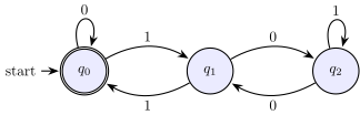
A deterministic finite automaton that accepts binary numbers divisible by 3, drawn with the TikZ automata library: an initial and accepting state, loops and bent transitions.
\usetikzlibrary{automata, positioning, arrows.meta}
\begin{tikzpicture}[
  shorten >=1pt, node distance=30mm, on grid, auto, thick,
  >={Stealth[length=2.6mm]},
  every state/.style={fill=blue!8, minimum size=11mm}
]
  \node[state, initial, accepting] (q0) {$q_0$};
  \node[state] (q1) [right=of q0] {$q_1$};
  \node[state] (q2) [right=of q1] {$q_2$};
  \path[->]
    (q0) edge [loop above] node {0} ()
         edge [bend left] node {1} (q1)
    (q1) edge [bend left] node {1} (q0)
         edge [bend left] node {0} (q2)
    (q2) edge [bend left] node {0} (q1)
         edge [loop above] node {1} ();
\end{tikzpicture}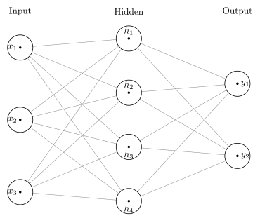
A fully connected network with three inputs, four hidden units and two outputs: every neuron wired to every neuron in the next layer, in three labelled columns.
A real answer from Forma's vector-graphics oracle, verified by vector-graphics@c738bf88.
\begin{tikzpicture}[x=1pt,y=1pt]
  \path[use as bounding box] (0,0) rectangle (278.54,237.56);
  \draw[draw=black!45,line width=0.4pt] (21.58,186.51) -- (138,196.21);
  \draw[draw=black!45,line width=0.4pt] (21.58,186.51) -- (138,138);
  \draw[draw=black!45,line width=0.4pt] (21.58,186.51) -- (138,79.79);
  \draw[draw=black!45,line width=0.4pt] (21.58,186.51) -- (138,21.58);
  \draw[draw=black!45,line width=0.4pt] (21.58,108.9) -- (138,196.21);
  \draw[draw=black!45,line width=0.4pt] (21.58,108.9) -- (138,138);
  \draw[draw=black!45,line width=0.4pt] (21.58,108.9) -- (138,79.79);
  \draw[draw=black!45,line width=0.4pt] (21.58,108.9) -- (138,21.58);
  \draw[draw=black!45,line width=0.4pt] (21.58,31.28) -- (138,196.21);
  \draw[draw=black!45,line width=0.4pt] (21.58,31.28) -- (138,138);
  \draw[draw=black!45,line width=0.4pt] (21.58,31.28) -- (138,79.79);
  \draw[draw=black!45,line width=0.4pt] (21.58,31.28) -- (138,21.58);
  \draw[draw=black!45,line width=0.4pt] (138,196.21) -- (254.42,147.7);
  \draw[draw=black!45,line width=0.4pt] (138,196.21) -- (254.42,70.09);
  \draw[draw=black!45,line width=0.4pt] (138,138) -- (254.42,147.7);
  \draw[draw=black!45,line width=0.4pt] (138,138) -- (254.42,70.09);
  \draw[draw=black!45,line width=0.4pt] (138,79.79) -- (254.42,147.7);
  \draw[draw=black!45,line width=0.4pt] (138,79.79) -- (254.42,70.09);
  \draw[draw=black!45,line width=0.4pt] (138,21.58) -- (254.42,147.7);
  \draw[draw=black!45,line width=0.4pt] (138,21.58) -- (254.42,70.09);
  \filldraw[draw=black,line width=0.6pt,fill=white] (21.58,186.51) circle[radius=13.58pt];
  \filldraw[draw=black,line width=0.6pt,fill=white] (21.58,108.9) circle[radius=13.58pt];
  \filldraw[draw=black,line width=0.6pt,fill=white] (21.58,31.28) circle[radius=13.58pt];
  \filldraw[draw=black,line width=0.6pt,fill=white] (138,196.21) circle[radius=13.58pt];
  \filldraw[draw=black,line width=0.6pt,fill=white] (138,138) circle[radius=13.58pt];
  \filldraw[draw=black,line width=0.6pt,fill=white] (138,79.79) circle[radius=13.58pt];
  \filldraw[draw=black,line width=0.6pt,fill=white] (138,21.58) circle[radius=13.58pt];
  \filldraw[draw=black,line width=0.6pt,fill=white] (254.42,147.7) circle[radius=13.58pt];
  \filldraw[draw=black,line width=0.6pt,fill=white] (254.42,70.09) circle[radius=13.58pt];
  \filldraw[draw=none,line width=0.4pt,fill=black] (21.58,186.51) circle[radius=1.3pt];
  \filldraw[draw=none,line width=0.4pt,fill=black] (21.58,108.9) circle[radius=1.3pt];
  \filldraw[draw=none,line width=0.4pt,fill=black] (21.58,31.28) circle[radius=1.3pt];
  \filldraw[draw=none,line width=0.4pt,fill=black] (138,196.21) circle[radius=1.3pt];
  \filldraw[draw=none,line width=0.4pt,fill=black] (138,138) circle[radius=1.3pt];
  \filldraw[draw=none,line width=0.4pt,fill=black] (138,79.79) circle[radius=1.3pt];
  \filldraw[draw=none,line width=0.4pt,fill=black] (138,21.58) circle[radius=1.3pt];
  \filldraw[draw=none,line width=0.4pt,fill=black] (254.42,147.7) circle[radius=1.3pt];
  \filldraw[draw=none,line width=0.4pt,fill=black] (254.42,70.09) circle[radius=1.3pt];
  \node[text=black,anchor=center,font=\fontsize{10pt}{12pt}\selectfont] at (21.58,225.31) {Input};
  \node[text=black,anchor=center,font=\fontsize{10pt}{12pt}\selectfont] at (138,225.31) {Hidden};
  \node[text=black,anchor=center,font=\fontsize{10pt}{12pt}\selectfont] at (254.42,225.31) {Output};
  \node[text=black,anchor=center,font=\fontsize{10pt}{12pt}\selectfont] at (13.19,186.51) {$x_{1}$};
  \node[text=black,anchor=center,font=\fontsize{10pt}{12pt}\selectfont] at (13.19,108.9) {$x_{2}$};
  \node[text=black,anchor=center,font=\fontsize{10pt}{12pt}\selectfont] at (13.19,31.28) {$x_{3}$};
  \node[text=black,anchor=center,font=\fontsize{10pt}{12pt}\selectfont] at (138,204.46) {$h_{1}$};
  \node[text=black,anchor=center,font=\fontsize{10pt}{12pt}\selectfont] at (138,146.25) {$h_{2}$};
  \node[text=black,anchor=center,font=\fontsize{10pt}{12pt}\selectfont] at (138,71.54) {$h_{3}$};
  \node[text=black,anchor=center,font=\fontsize{10pt}{12pt}\selectfont] at (138,13.33) {$h_{4}$};
  \node[text=black,anchor=center,font=\fontsize{10pt}{12pt}\selectfont] at (262.81,147.7) {$y_{1}$};
  \node[text=black,anchor=center,font=\fontsize{10pt}{12pt}\selectfont] at (262.81,70.09) {$y_{2}$};
\end{tikzpicture}
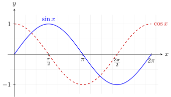
sin x and cos x from 0 to 2π, drawn with TikZ plot over a domain, on a grid with arrowed axes and tick labels at multiples of π. No pgfplots needed.
\begin{tikzpicture}[x=1.15cm, y=1.6cm, >=stealth]
  \draw[very thin, gray!30, step=0.5] (-0.2,-1.3) grid (6.6,1.3);
  \draw[->] (-0.3,0) -- (6.8,0) node[right] {$x$};
  \draw[->] (0,-1.4) -- (0,1.5) node[above] {$y$};
  \foreach \x/\l in {1.5708/{\frac{\pi}{2}}, 3.1416/{\pi}, 4.7124/{\frac{3\pi}{2}}, 6.2832/{2\pi}}
    \draw (\x,0.05) -- (\x,-0.05) node[below] {$\l$};
  \foreach \y in {-1, 1}
    \draw (0.05,\y) -- (-0.05,\y) node[left] {$\y$};
  \draw[thick, blue, domain=0:6.2832, samples=120, smooth] plot (\x, {sin(\x r)});
  \draw[thick, red!80!black, dashed, domain=0:6.2832, samples=120, smooth] plot (\x, {cos(\x r)});
  \node[blue, above] at (1.5708,1.02) {$\sin x$};
  \node[red!80!black, right] at (6.3,1) {$\cos x$};
\end{tikzpicture}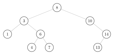
The keys 8, 3, 10, 1, 6, 14, 4, 7, 13 inserted in order. Read the nodes left to right and they come out sorted, which is what makes it a search tree.
A real answer from Forma's vector-graphics oracle, verified by vector-graphics@c738bf88.
\begin{tikzpicture}[x=1pt,y=1pt]
  \path[use as bounding box] (0,0) rectangle (276,132.15);
  \draw[draw=black!45,line width=0.4pt] (138,114.02) -- (58.08,82.06);
  \draw[draw=black!45,line width=0.4pt] (138,114.02) -- (217.92,82.06);
  \draw[draw=black!45,line width=0.4pt] (58.08,82.06) -- (18.12,50.09);
  \draw[draw=black!45,line width=0.4pt] (58.08,82.06) -- (98.04,50.09);
  \draw[draw=black!45,line width=0.4pt] (98.04,50.09) -- (76.73,18.12);
  \draw[draw=black!45,line width=0.4pt] (98.04,50.09) -- (119.35,18.12);
  \draw[draw=black!45,line width=0.4pt] (217.92,82.06) -- (257.88,50.09);
  \draw[draw=black!45,line width=0.4pt] (257.88,50.09) -- (236.57,18.12);
  \filldraw[draw=black,line width=0.6pt,fill=white] (138,114.02) circle[radius=10.12pt];
  \filldraw[draw=black,line width=0.6pt,fill=white] (58.08,82.06) circle[radius=10.12pt];
  \filldraw[draw=black,line width=0.6pt,fill=white] (217.92,82.06) circle[radius=10.12pt];
  \filldraw[draw=black,line width=0.6pt,fill=white] (18.12,50.09) circle[radius=10.12pt];
  \filldraw[draw=black,line width=0.6pt,fill=white] (98.04,50.09) circle[radius=10.12pt];
  \filldraw[draw=black,line width=0.6pt,fill=white] (257.88,50.09) circle[radius=10.12pt];
  \filldraw[draw=black,line width=0.6pt,fill=white] (76.73,18.12) circle[radius=10.12pt];
  \filldraw[draw=black,line width=0.6pt,fill=white] (119.35,18.12) circle[radius=10.12pt];
  \filldraw[draw=black,line width=0.6pt,fill=white] (236.57,18.12) circle[radius=10.12pt];
  \node[text=black,anchor=center,font=\fontsize{10pt}{12pt}\selectfont] at (138,114.02) {8};
  \node[text=black,anchor=center,font=\fontsize{10pt}{12pt}\selectfont] at (58.08,82.06) {3};
  \node[text=black,anchor=center,font=\fontsize{10pt}{12pt}\selectfont] at (217.92,82.06) {10};
  \node[text=black,anchor=center,font=\fontsize{10pt}{12pt}\selectfont] at (18.12,50.09) {1};
  \node[text=black,anchor=center,font=\fontsize{10pt}{12pt}\selectfont] at (98.04,50.09) {6};
  \node[text=black,anchor=center,font=\fontsize{10pt}{12pt}\selectfont] at (257.88,50.09) {14};
  \node[text=black,anchor=center,font=\fontsize{10pt}{12pt}\selectfont] at (76.73,18.12) {4};
  \node[text=black,anchor=center,font=\fontsize{10pt}{12pt}\selectfont] at (119.35,18.12) {7};
  \node[text=black,anchor=center,font=\fontsize{10pt}{12pt}\selectfont] at (236.57,18.12) {13};
\end{tikzpicture}
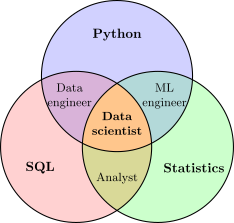
Three overlapping sets with every overlap filled in its own colour by clipping one circle to another, and each region labelled.
\begin{tikzpicture}[thick]
  \def\r{2cm}
  \def\A{(90:1.25cm) circle (\r)}
  \def\B{(210:1.25cm) circle (\r)}
  \def\C{(330:1.25cm) circle (\r)}
  % each set, then each overlap, filled by clipping one circle to another
  \fill[blue!18] \A;  \fill[red!18] \B;  \fill[green!20] \C;
  \begin{scope} \clip \A; \fill[violet!30] \B; \end{scope}
  \begin{scope} \clip \A; \fill[teal!30] \C; \end{scope}
  \begin{scope} \clip \B; \fill[olive!30] \C; \end{scope}
  \begin{scope} \clip \A; \clip \B; \fill[orange!45] \C; \end{scope}
  \draw \A \B \C;
  \node[font=\bfseries] at (90:2.35cm) {Python};
  \node[font=\bfseries] at (210:2.35cm) {SQL};
  \node[font=\bfseries] at (330:2.35cm) {Statistics};
  \node[font=\small, align=center] at (150:1.45cm) {Data\\engineer};
  \node[font=\small, align=center] at (30:1.45cm) {ML\\engineer};
  \node[font=\small] at (270:1.45cm) {Analyst};
  \node[font=\small\bfseries, align=center] at (0,0) {Data\\scientist};
\end{tikzpicture}02 About TikZ
TikZ is the drawing language of LaTeX: you describe a figure in coordinates and nodes, and TeX places every line and label exactly. It is how most diagrams in papers and textbooks are made, from trees and graphs to commutative diagrams and circuits.
No. Paste the tikzpicture environment only; the renderer supplies the document around it. A \usetikzlibrary line at the top of what you paste is loaded too, so positioning, arrows.meta and the other libraries work.
LaTeX with the TikZ package, then dvisvgm to turn the page into SVG, with text set as outlines so the file looks the same everywhere. It runs in a sandbox with no network and keeps nothing you send.
The editor shows TeX's own error line, such as an undefined control sequence. Shell escape and reading files are switched off, so a figure that needs either will not draw.