Which trace types are supported?
The 2D ones in Plotly.js: scatter, bar, box, violin, histogram, 2D histogram, heatmap, contour and pie. 3D, map and Sankey traces are not loaded, and the editor says so if a figure uses one.
Tools · Plotly
Paste a Plotly figure, its data and layout as JSON, and see it drawn by Plotly.js. It runs in your browser and the figure is not sent anywhere; download the chart as SVG or PNG.
Or describe it in words and get source you can edit, checked before you see it.
Part of Forma Visuals: Chart your data · For developers
Correlation heatmap A correlation matrix as a Plotly heatmap: a diverging RdBu scale fixed from -1 to 1 with zmin and zmax, and every cell labelled with its value by texttemplate. Illustrative data.
In your browser, drawn with Plotly.js (MIT), Apache ECharts (Apache-2.0, notice), Chart.js (MIT).
01 Examples
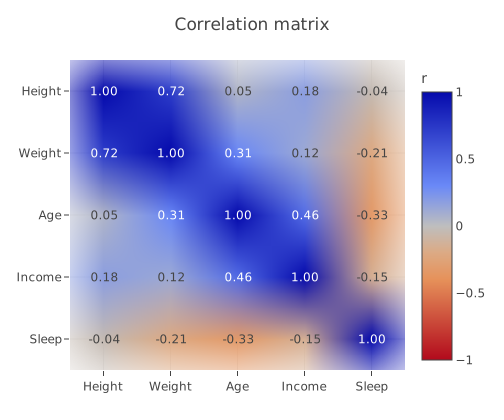
A correlation matrix as a Plotly heatmap: a diverging RdBu scale fixed from -1 to 1 with zmin and zmax, and every cell labelled with its value by texttemplate. Illustrative data.
{
  "data": [
    {
      "type": "heatmap",
      "x": [
        "Height",
        "Weight",
        "Age",
        "Income",
        "Sleep"
      ],
      "y": [
        "Height",
        "Weight",
        "Age",
        "Income",
        "Sleep"
      ],
      "z": [
        [
          1,
          0.72,
          0.05,
          0.18,
          -0.04
        ],
        [
          0.72,
          1,
          0.31,
          0.12,
          -0.21
        ],
        [
          0.05,
          0.31,
          1,
          0.46,
          -0.33
        ],
        [
          0.18,
          0.12,
          0.46,
          1,
          -0.15
        ],
        [
          -0.04,
          -0.21,
          -0.33,
          -0.15,
          1
        ]
      ],
      "zmin": -1,
      "zmax": 1,
      "colorscale": "RdBu",
      "reversescale": true,
      "texttemplate": "%{z:.2f}",
      "colorbar": {
        "title": {
          "text": "r"
        }
      }
    }
  ],
  "layout": {
    "title": {
      "text": "Correlation matrix"
    },
    "yaxis": {
      "autorange": "reversed"
    },
    "margin": {
      "l": 70,
      "r": 20,
      "t": 60,
      "b": 50
    }
  }
}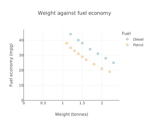
Car weight against fuel economy for petrol and diesel cars, two Plotly scatter traces in marker mode with a legend: the figure exactly as Forma wrote it from the prompt.
A real answer from Forma's chart oracle, verified by chart@6baf09f0.
{
  "data": [
    {
      "type": "scatter",
      "mode": "markers",
      "x": [
        1.2,
        1.4,
        1.5,
        1.7,
        1.9,
        2.1,
        2.3
      ],
      "y": [
        44,
        40,
        38,
        34,
        31,
        28,
        25
      ],
      "name": "Diesel",
      "marker": {
        "symbol": "circle-open"
      }
    },
    {
      "type": "scatter",
      "mode": "markers",
      "x": [
        1.1,
        1.2,
        1.3,
        1.4,
        1.5,
        1.6,
        1.8,
        2,
        2.2
      ],
      "y": [
        38,
        35,
        33,
        31,
        29,
        27,
        24,
        21,
        19
      ],
      "name": "Petrol",
      "marker": {
        "symbol": "circle-open"
      }
    }
  ],
  "layout": {
    "title": {
      "text": "Weight against fuel economy"
    },
    "xaxis": {
      "title": {
        "text": "Weight (tonnes)"
      },
      "type": "linear",
      "rangemode": "tozero"
    },
    "yaxis": {
      "title": {
        "text": "Fuel economy (mpg)"
      },
      "type": "linear",
      "rangemode": "tozero"
    },
    "legend": {
      "title": {
        "text": "Fuel"
      }
    }
  }
}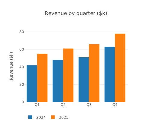
Quarterly revenue for two years side by side: two Plotly bar traces with barmode set to group and the legend moved below the chart. Illustrative data.
{
  "data": [
    {
      "type": "bar",
      "name": "2024",
      "x": [
        "Q1",
        "Q2",
        "Q3",
        "Q4"
      ],
      "y": [
        42,
        48,
        51,
        63
      ]
    },
    {
      "type": "bar",
      "name": "2025",
      "x": [
        "Q1",
        "Q2",
        "Q3",
        "Q4"
      ],
      "y": [
        55,
        61,
        66,
        78
      ]
    }
  ],
  "layout": {
    "title": {
      "text": "Revenue by quarter ($k)"
    },
    "barmode": "group",
    "yaxis": {
      "title": {
        "text": "Revenue ($k)"
      }
    },
    "legend": {
      "orientation": "h",
      "y": -0.15
    }
  }
}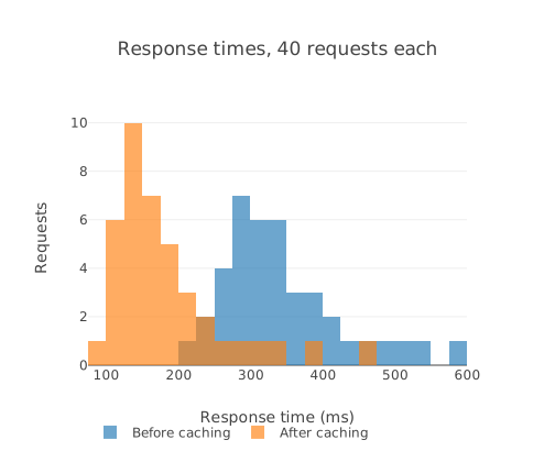
Response times before and after adding a cache, as two Plotly histogram traces with the same xbins, overlaid with barmode overlay and some opacity so both show. Illustrative data.
{
  "data": [
    {
      "type": "histogram",
      "name": "Before caching",
      "x": [
        212,
        238,
        245,
        251,
        260,
        264,
        271,
        275,
        279,
        283,
        288,
        291,
        294,
        298,
        301,
        305,
        309,
        312,
        316,
        321,
        325,
        329,
        334,
        338,
        343,
        349,
        356,
        362,
        370,
        377,
        385,
        396,
        408,
        421,
        437,
        455,
        478,
        506,
        541,
        590
      ],
      "xbins": {
        "start": 50,
        "end": 650,
        "size": 25
      },
      "opacity": 0.65
    },
    {
      "type": "histogram",
      "name": "After caching",
      "x": [
        96,
        104,
        109,
        113,
        117,
        120,
        123,
        126,
        128,
        131,
        133,
        136,
        138,
        141,
        143,
        146,
        149,
        151,
        154,
        157,
        160,
        163,
        167,
        171,
        175,
        179,
        184,
        190,
        196,
        203,
        211,
        220,
        231,
        244,
        259,
        278,
        302,
        335,
        380,
        452
      ],
      "xbins": {
        "start": 50,
        "end": 650,
        "size": 25
      },
      "opacity": 0.65
    }
  ],
  "layout": {
    "title": {
      "text": "Response times, 40 requests each"
    },
    "barmode": "overlay",
    "xaxis": {
      "title": {
        "text": "Response time (ms)"
      }
    },
    "yaxis": {
      "title": {
        "text": "Requests"
      }
    },
    "legend": {
      "orientation": "h",
      "y": -0.2
    }
  }
}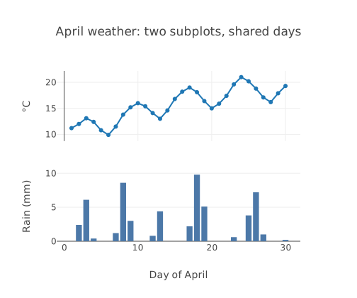
Daily temperature as a line and rainfall as bars in two stacked subplots sharing the day axis, laid out with layout.grid and a second x and y axis. Illustrative data.
{
  "data": [
    {
      "type": "scatter",
      "mode": "lines+markers",
      "name": "Temperature",
      "x": [
        1,
        2,
        3,
        4,
        5,
        6,
        7,
        8,
        9,
        10,
        11,
        12,
        13,
        14,
        15,
        16,
        17,
        18,
        19,
        20,
        21,
        22,
        23,
        24,
        25,
        26,
        27,
        28,
        29,
        30
      ],
      "y": [
        11.2,
        12,
        13.1,
        12.4,
        10.8,
        9.9,
        11.5,
        13.8,
        15.2,
        16,
        15.4,
        14.1,
        13,
        14.6,
        16.8,
        18.2,
        19,
        18.1,
        16.4,
        15,
        15.9,
        17.4,
        19.6,
        21,
        20.2,
        18.8,
        17.1,
        16.2,
        17.9,
        19.3
      ],
      "xaxis": "x",
      "yaxis": "y"
    },
    {
      "type": "bar",
      "name": "Rainfall",
      "x": [
        1,
        2,
        3,
        4,
        5,
        6,
        7,
        8,
        9,
        10,
        11,
        12,
        13,
        14,
        15,
        16,
        17,
        18,
        19,
        20,
        21,
        22,
        23,
        24,
        25,
        26,
        27,
        28,
        29,
        30
      ],
      "y": [
        0,
        2.4,
        6.1,
        0.4,
        0,
        0,
        1.2,
        8.6,
        3,
        0,
        0,
        0.8,
        4.4,
        0,
        0,
        0,
        2.2,
        9.8,
        5.1,
        0,
        0,
        0,
        0.6,
        0,
        3.8,
        7.2,
        1,
        0,
        0,
        0.2
      ],
      "xaxis": "x2",
      "yaxis": "y2",
      "marker": {
        "color": "#4c78a8"
      }
    }
  ],
  "layout": {
    "title": {
      "text": "April weather: two subplots, shared days"
    },
    "showlegend": false,
    "grid": {
      "rows": 2,
      "columns": 1,
      "pattern": "independent",
      "roworder": "top to bottom"
    },
    "xaxis": {
      "matches": "x2",
      "showticklabels": false
    },
    "yaxis": {
      "title": {
        "text": "°C"
      }
    },
    "xaxis2": {
      "title": {
        "text": "Day of April"
      }
    },
    "yaxis2": {
      "title": {
        "text": "Rain (mm)"
      }
    }
  }
}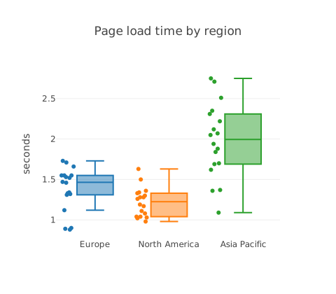
Page load times for three regions as box plots with every point shown beside its box, to compare the spread as well as the middle. Illustrative data.
{
  "data": [
    {
      "type": "box",
      "name": "Europe",
      "y": [
        1.32,
        1.55,
        1.33,
        1.31,
        1.12,
        1.34,
        1.73,
        1.53,
        1.71,
        1.47,
        1.52,
        1.46,
        0.9,
        1.66,
        1.55,
        1.55,
        0.89,
        0.88
      ],
      "boxpoints": "all",
      "jitter": 0.4
    },
    {
      "type": "box",
      "name": "North America",
      "y": [
        0.98,
        1.08,
        1.28,
        1.19,
        1.33,
        1.04,
        1.28,
        1.3,
        1.03,
        1.63,
        1.34,
        1.5,
        1.04,
        1.02,
        1.11,
        1.17,
        1.36,
        1.26
      ],
      "boxpoints": "all",
      "jitter": 0.4
    },
    {
      "type": "box",
      "name": "Asia Pacific",
      "y": [
        1.88,
        1.62,
        1.84,
        2.71,
        1.7,
        2.22,
        2.31,
        1.36,
        2.12,
        2.75,
        1.09,
        1.94,
        2.05,
        1.69,
        2.35,
        2.07,
        1.37,
        2.51
      ],
      "boxpoints": "all",
      "jitter": 0.4
    }
  ],
  "layout": {
    "title": {
      "text": "Page load time by region"
    },
    "yaxis": {
      "title": {
        "text": "seconds"
      }
    },
    "showlegend": false
  }
}02 About Plotly
Plotly describes a chart as a list of traces plus a layout. The same JSON draws in Plotly for Python, R and JavaScript, so a figure written or generated once can be shown anywhere.
The 2D ones in Plotly.js: scatter, bar, box, violin, histogram, 2D histogram, heatmap, contour and pie. 3D, map and Sankey traces are not loaded, and the editor says so if a figure uses one.
Yes, as JSON: in Python, fig.to_json() gives exactly the data and layout this editor reads.
No. Plotly charts are drawn in a sandboxed frame on this page, which cannot reach the network or your storage.