What about set terminal and set output?
The renderer chooses the terminal itself and draws to SVG, so lines such as set terminal pngcairo and set output are ignored; set terminal svg size W,H is kept, so a script can still set its size.
Tools · gnuplot
Paste a gnuplot script and get the plot back without installing anything. Functions, parametric curves, 3D surfaces with splot and inline data blocks all work; download the result as SVG or PNG.
Or describe it in words and get source you can edit, checked before you see it.
Part of Forma Visuals: Chart your data · For students and scientists
Histogram Sixty exam scores, one per line in a data block, counted into five-mark bins with a bin() function and smooth freq, then drawn with boxes. The usual way to make a histogram in gnuplot.
In your browser, drawn with Plotly.js (MIT), Apache ECharts (Apache-2.0, notice), Chart.js (MIT).
01 Examples
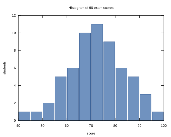
Sixty exam scores, one per line in a data block, counted into five-mark bins with a bin() function and smooth freq, then drawn with boxes. The usual way to make a histogram in gnuplot.
# 60 exam scores, one per line, counted into bands 5 marks wide
$scores << EOD
42
47
51
53
55
56
58
58
59
61
61
62
63
63
64
65
65
66
66
67
67
68
68
69
69
70
70
71
71
72
72
72
73
73
74
74
75
75
76
76
77
77
78
79
79
80
81
82
82
83
84
85
86
87
88
89
91
92
94
97
EOD
set title 'Histogram of 60 exam scores'
set xlabel 'score'
set ylabel 'students'
width = 5
bin(x) = width * floor(x / width) + width / 2.0
set boxwidth width * 0.92
set style fill solid 0.7 border lc rgb '#204a87'
set xrange [40:100]
set yrange [0:*]
set xtics 40, 10, 100
unset key
plot $scores using (bin($1)):(1.0) smooth freq with boxes lc rgb '#3465a4'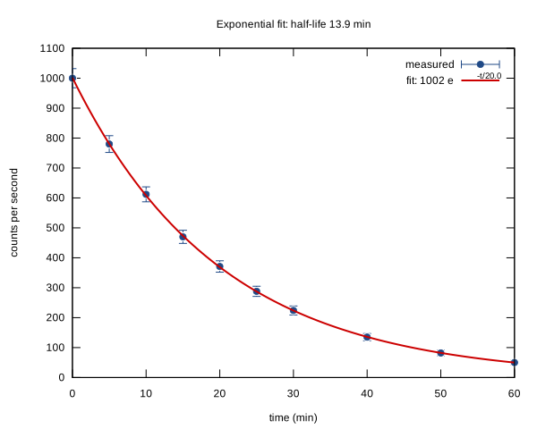
Decay measurements plotted with yerrorbars and fitted to an exponential with fit, weighted by the errors; the fitted constants and the half-life go into the key and title with sprintf.
# Measured activity of a radioactive sample, with the counting error on each point
$decay << EOD
0   1000 32
5    780 28
10   612 25
15   470 22
20   371 19
25   288 17
30   224 15
40   135 12
50    82  9
60    50  7
EOD
set fit quiet nolog
f(t) = a * exp(-t / tau)
a = 1000; tau = 20
fit f(x) $decay using 1:2:3 yerrors via a, tau
set title sprintf('Exponential fit: half-life %.1f min', tau * log(2))
set xlabel 'time (min)'
set ylabel 'counts per second'
set key top right
plot $decay using 1:2:3 with yerrorbars pt 7 ps 0.8 lc rgb '#204a87' title 'measured', \
     f(x) lw 2 lc rgb '#cc0000' title sprintf('fit: %.0f e^{-t/%.1f}', a, tau)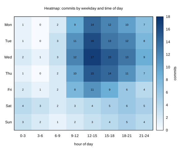
Commits by weekday and time of day read as a matrix from a data block, drawn as coloured cells with a palette and each value printed on top with labels.
# Average commits per hour block (columns) for each weekday (rows)
$commits << EOD
1 0 2 9 14 12 10 7
1 0 3 11 16 13 12 8
2 1 3 12 17 15 13 9
1 0 2 10 15 14 11 7
2 1 2 8 11 9 6 4
4 3 2 3 4 5 6 5
3 2 1 2 3 4 5 4
EOD
set title 'Heatmap: commits by weekday and time of day'
set xtics ('0-3' 0, '3-6' 1, '6-9' 2, '9-12' 3, '12-15' 4, '15-18' 5, '18-21' 6, '21-24' 7)
set ytics ('Mon' 0, 'Tue' 1, 'Wed' 2, 'Thu' 3, 'Fri' 4, 'Sat' 5, 'Sun' 6)
set yrange [6.5:-0.5]
set xrange [-0.5:7.5]
set xlabel 'hour of day'
set cblabel 'commits'
set palette defined (0 '#f7fbff', 0.5 '#6baed6', 1 '#08306b')
set tics scale 0
unset key
plot $commits matrix using 1:2:(0.5):(0.5):3 with boxxyerror fs solid noborder lc palette, \
     $commits matrix using 1:2:(sprintf('%d', $3)) with labels font ',9'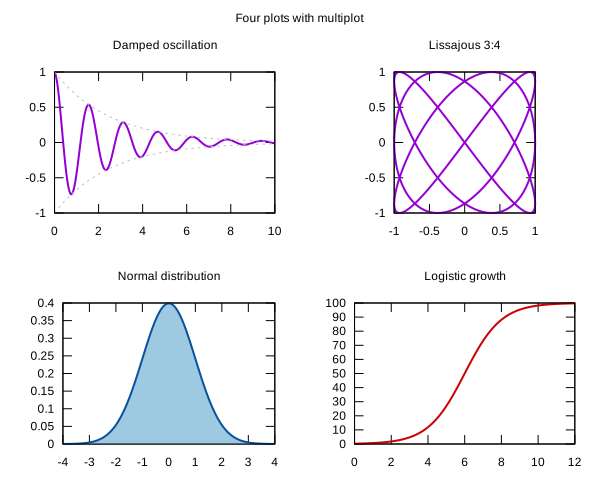
Four plots on one page with set multiplot layout 2, 2: a damped oscillation, a Lissajous curve, a filled normal distribution and a logistic curve.
# Four plots on one page with multiplot
set multiplot layout 2, 2 title 'Four plots with multiplot'
set samples 400
unset key

set title 'Damped oscillation'
plot [0:10] exp(-0.4*x) * cos(4*x) lw 2, exp(-0.4*x) dt 2 lc rgb 'gray', -exp(-0.4*x) dt 2 lc rgb 'gray'

set title 'Lissajous 3:4'
set parametric
set size ratio -1
set xtics 0.5
set ytics 0.5
plot [0:2*pi] sin(3*t + pi/2), sin(4*t) lw 2
unset parametric
set size noratio
set xtics autofreq
set ytics autofreq

set title 'Normal distribution'
plot [-4:4] exp(-x**2 / 2) / sqrt(2*pi) with filledcurves y1=0 lc rgb '#9ecae1', exp(-x**2 / 2) / sqrt(2*pi) lw 2 lc rgb '#08519c'

set title 'Logistic growth'
plot [0:12] 100 / (1 + exp(-(x - 6))) lw 2 lc rgb '#cc0000'

unset multiplot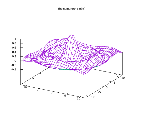
sin(r)/r as a 3D wireframe with hidden lines removed: the classic surface for showing off gnuplot's splot.
set title 'The sombrero: sin(r)/r'
set hidden3d
set isosamples 30, 30
set xrange [-12:12]
set yrange [-12:12]
set view 60, 30
unset key
r(x,y) = sqrt(x**2 + y**2) + 1e-9
splot sin(r(x,y)) / r(x,y) with lines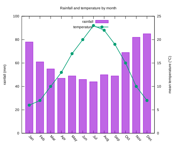
Monthly rainfall as bars and mean temperature as a line on a second axis, from inline values held in a gnuplot data block. Illustrative data.
$climate << EOD
Jan 78 6
Feb 61 7
Mar 55 10
Apr 47 13
May 49 17
Jun 46 20
Jul 44 23
Aug 50 22
Sep 49 19
Oct 69 15
Nov 82 10
Dec 85 7
EOD
set title 'Rainfall and temperature by month'
set style fill solid 0.6
set boxwidth 0.7
set ylabel 'rainfall (mm)'
set y2label 'mean temperature (°C)'
set y2tics
set ytics nomirror
set yrange [0:100]
set y2range [0:25]
set key top center
set xtics rotate by -45
plot $climate using 0:2:xtic(1) with boxes title 'rainfall', \
$climate using 0:3 axes x1y2 with linespoints lw 2 pt 7 title 'temperature'02 About gnuplot
gnuplot is a command-line plotting program that has drawn scientific graphs since 1986. A few lines describe a plot of a function, a data file or a surface, which is why it is still a favourite for papers, lab notes and quick looks at data.
The renderer chooses the terminal itself and draws to SVG, so lines such as set terminal pngcairo and set output are ignored; set terminal svg size W,H is kept, so a script can still set its size.
Not from disk. Put the data inline in a data block ($data << EOD … EOD) and plot $data, as in the histogram example.
No. The script runs in a sandbox with no shell, no network and no access to files outside its own folder, and nothing you send is kept.